Insert Check Mark in Excel

You can insert a check mark (aka. tick mark) in Excel by using the font “Wingdings 2” or inserting a symbol. These static symbols are useful to make an eye-catching to-do list.

1. Select cell D3 and press SHFT + P on your keyboard.

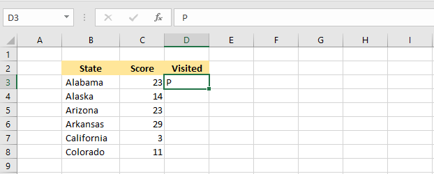
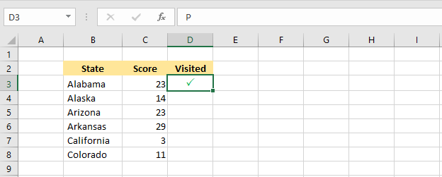
2. Select Font “Wingdings 2” on the Home tab.

Apply other formatting: font size-13; font color-green; alignment- center

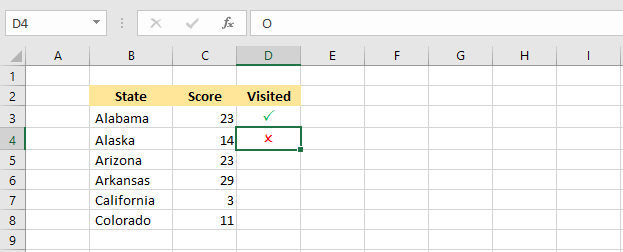
3. To insert a CROSS check mark, select cell D4 and press SHFT + O.

Apply other formatting: font size-13; font color-red; alignment- center

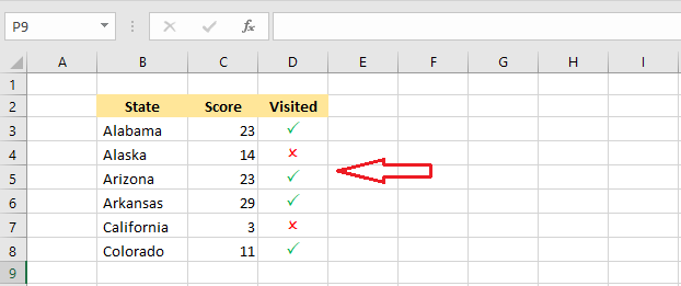
4. To create a to-do list, just Copy (CTRL+c) and Paste (CTRL+v) in the cells below.

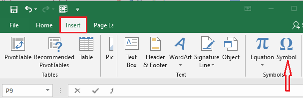
5. To insert such check marks from the symbol, click “Symbol” on the Insert tab.

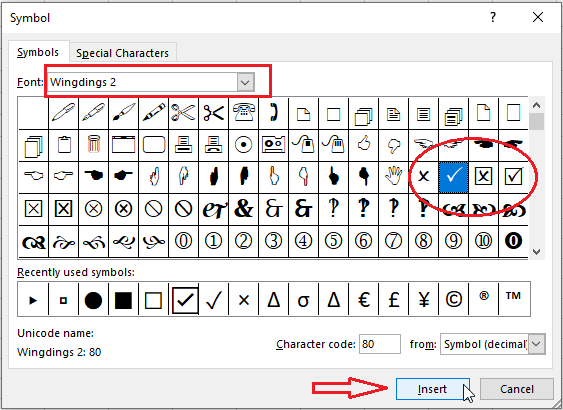
6. Change font to “Wingdings 2” from the drop-down list.

7. Select any symbol you like and then click “Insert.”

Note: You now know how to insert check marks in Excel. This will help you create a beautiful to-do list or task planner.

14 of 14 Completed! Congrats!! You can now move on to Ch05: Next Example >>

<< Previous Example | Skip to Next Chapter 05: Formulas and Functions Basics