
The formulas used to find the nearest values in Excel are tricky. It is a more complicated job than finding matching values.
There are two ways to find the closest match from a data set in Excel:
- The INDEX-MATCH Formula
- The XLOOKUP Formula
To better understand how these formulas work, let’s consider the following dataset and find the closest value in that dataset:
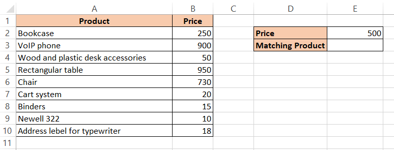
In the above dataset, each item has a unique price. We want to find the closest price to the price in cell E2. The closest price can be higher or lower than the price in cell E2, but it has to be the nearest price.
Let’s see how to do that using the following formulas.
1. The INDEX-MATCH Formula:
This formula is the combination of INDEX and MATCH functions in Excel. Although these functions are not that useful alone, they are powerful when merged into one formula.
Basically, the MATCH function provides the “index” of an item in a range of cells, whereas the INDEX function provides the contents at a given index. But the combination of this two help find a value in a cell from a table and return that value in another cell in the same row or column.
How to find the Closest value:
Here, we can use a formula, which includes the ABS, MIN, and MATCH functions as given below.
{=INDEX(A2:A10,MATCH(MIN(ABS(B2:B10-E2)), ABS(B2:B10-E2),0))}
Since it is an array formula, in order to get the accurate result from this function, do not write down the curly braces that wrap the whole formula and press the CTRL+SHIFT+ENTER shortcut from the keyboard. In this way, the above formula will return the product with the price closest to the price in cell E2, in the cell range B2:B10.
For example, let’s see how to use this formula to find the product with the closest value to the value in cell E2.
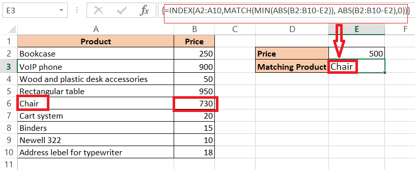
In the picture, the formula returned “Chair” as the closest valued item in cell E3, since the price of Chair (730) is the closest price to the number 500 in cell E2.
Note: If the list consists of two numbers that are equally closest to the lookup number, the formula will return the first item in the result box.
Breaking down the above Formula:
If you want to understand how the formula works, this section is for you.
Let’s discuss the innermost function, first:
- B2:B10-E2
It subtracts the value in cell E2 from each value in the range B2:B10. Since it is an array operation, it returns an array of 8 values containing each of the differences. For example:
{-250;400;-450;450;230;-480;-485;-490;-482}
Here, some values are negative, because the values are smaller than 500.
- ABS(B2:B10-E2)
Since the formula wants to return the closest value without considering the fact that the number may be greater or less than the number in E2, the above formula converts all the values into absolute values. For example,
{250;400;450;450;230;480;485;490;482}
- MIN(ABS(B2:B10-E2)
After finding out the differences in values from the value in cell E2, the above formula searches the number that is the smallest difference. For example, we get the number 230. This is called the MIN function.
- MATCH(MIN(ABS(B2:B10-E2)), ABS(B2:B10-E2),0)
This MATCH function returns the relative position of the above value (230). For example, the item of the closest value is in the 5th position in the list. So this function returns the value 5.
- INDEX(A2:A10,MATCH(MIN(ABS(B2:B10-E2)), ABS(B2:B10-E2),0))
Finally, the INDEX Function finds out the item in the 5th position in the list. For example, the 5th item in the list is “Chair”. (Note- if there is another item having the same difference in values, the formula would show the first item in its result box).
2. The XLOOKUP Formula:
This method is very simple and used only in Excel 365 and in newer versions. It does not need the ABS and MIN functions. Hence, it is simple and easy.
Basically, it is a modern version of VLOOKUP, HLOOKUP, etc, meaning it can perform both vertical and horizontal lookups. It also supports different types of matching algorithms, for example, exact matching, approximate matching, partial matching, etc.
The advantage of this function is that it does not require sorted data to perform its task.
Let’s understand the function syntax first. The function syntax is:
XLOOKUP (lookup_value, lookup_array, return_array, [not_found], [match_mode], [search_mode])
Here,
- lookup_value is the value that we want to search.
- lookup_array means the range or array that we want to search in.
- return_array means the array from which we want to return the value corresponding to the matched item
- not_found means the value we want to return if there is no match. By default it is a blank string.
- match_mode means an integer representing the type of matching we want. (The possible values could be 0-default, 1- next larger value, -1- next smaller value, and 2- wildcard match.)
- search_mode means an integer that represents the order of the search. (The possible values of the parameter could be 1- search from the first item, -1- search from the last item, 2- binary search in ascending order, and -2- binary search in descending order.)
Now, let’s look at how this function actually works:
- The XLOOKUP function searches the lookup_array for the lookup_value and returns the value in the return_array.
- To perform searching and matching, it uses the optional parameters of the match_mode and the search_mode.
- If the function does not find any match, it returns the text in the not_found parameter. If this parameter is not specified, it returns a blank.
Following is the XLOOKUP function used in our example:
=XLOOKUP(E2,B2:B10,A2:A10,,1)
Here, we kept the not_found parameter blank, but if you do not want to keep it blank then you can write down any words that are suitable.
We also did not specify the 6th parameter, because we want the default search mode to work and search from the top.
The above function is applied to our dataset and we got the results below:
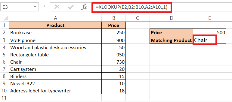
As we can see, our result is similar to the one using the first formula.
Thus far, we showed you how to find the closest match by using two formulas. Hope our discussion will help solve your problems in Excel. Thank you!