Excel is one of the useful platforms for handling survey data. Sometimes, a survey questionnaire includes only “Yes” or “No” responses from the participants.
A common question generally asked is how to count the number or percentage of the response “Yes” from that dataset. One way to solve this problem is to use the COUNTIF function in Excel.
Note that, “Yes” can be in the text form or a ticked checkbox.
Let’s discuss the function first.
The COUNTIF Function:
The COUNTIF function counts the number of cells in a given range that match a given condition. This function basically goes through each cell in the range and counts the cells that match the given condition.
The syntax for the function is:
=COUNTIF(range,condition)
Here,
- “range” is the range of cells that we want the function to work on.
- “condition” is the feature that should be present in a cell for that cell to be counted.
1. When the “Yes” is written as a text:
Now, we will see how to use the COUNTIF formula, when “Yes” is written as a text form in the cells.
Let’s look at the following dataset:
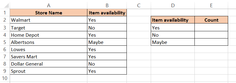
In the above dataset, we want to see whether the store listed have a certain item. We wrote “Yes” when the item is available in that particular store and “No” when the item is not available in that store. We also wrote “Maybe” for those stores, which sells the item seasonally.
If we want to know the list of stores that have a “Yes” response, we can use the COUNTIF formula.
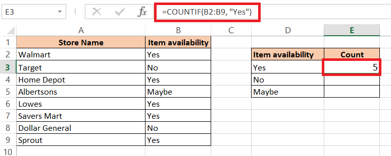
Here, we will count the cells that contain the “Yes” response from our range B2:B9.
To do that, let’s enter the following formula in cell E3:
=COUNTIF(B2:B9, “Yes”)
Following is the result we got:
Note: The COUNTIF formula is not case-insensitive, which means that it will count all the “Yes” regardless of the upper or lower case letter.
In the same way, if we want to know the number of cells that contain “No”, we need to write down “no” in place of “yes” in the above formula.
For example:

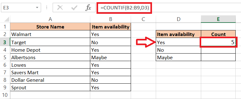
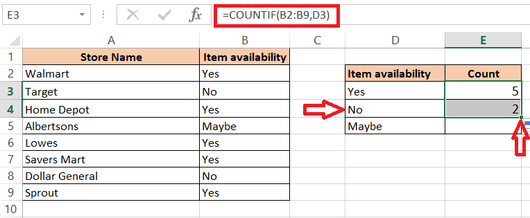
Alternatively, we can use the cell reference in place of the criteria in the formula. For example, we will replace the word “yes” with the cell reference (D3) in the following formula:
=COUNTIF(B2:B9,D3)
This means that the criterion in cell D3 will be the criteria in the formula. So the formula will return the number of cells that have the criteria specified in cell D3.
This technique (writing cell references other than the criteria itself) has an advantage. It makes the formula easier and quicker.
For example, to count the cells that contain “No”, we don’t need to rewrite the formula in cell E4. Simply, we have to select cell E3 and drag down the square button in the right corner of the cell boundary to cell E4. The formula will automatically include the criteria of cell D4. Hence, it will show the number of cells that have “no” response.
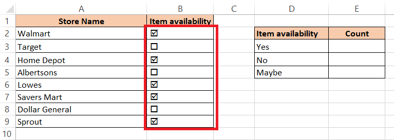
2. When “Yes” is written as a Ticked Checkbox:
Sometimes, the survey dataset has a checkbox instead of “Yes” or “No” options. If the checkbox is ticked it means “Yes”, and if the checkbox is empty it means “No”.
Let’s see what the dataset looks like with ticked checkboxes:
To find out how many have the item available, we need to count the number of cells that have ticked the checkbox.
But we cannot use any formula that will work for checkboxes. So we have to do some extra steps.
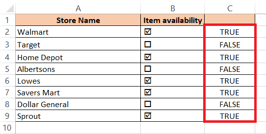
For example, we need to create a column called the “Helper” column, which will link its cells to the cells of column B. That means the cells will be linked to the checkboxes. Whenever a checkbox is ticked, the linked cell of the “helper” column will show a TRUE value. If the checkbox is left empty, the linked cell of the “helper” column will show the FALSE value. After getting these TRUE and FALSE values, we can use the COUNTIF formula.
In the example, let’s go through the process step by step:
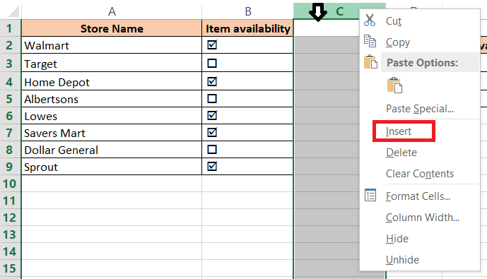
- Next to column B, we created another column by right clicking on the header of column C. A context bar appeared where we selected “Insert” option. Now, we can see that column C is selected.
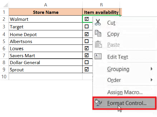
- Next, we right-click on one checkbox and select “Format Control”.
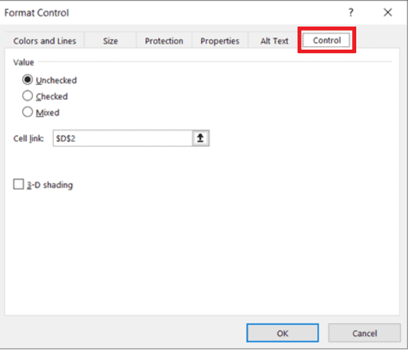
- Next, we selected the Control option from the Format Object dialog box.
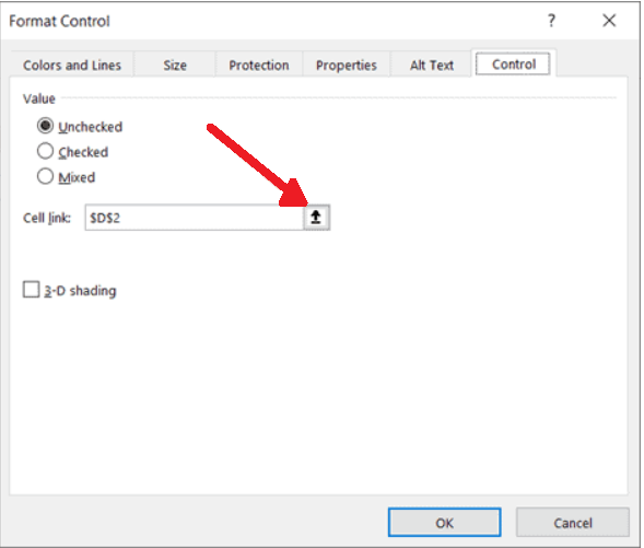
- Next, we clicked the right button of the Cell link.
- Now we select cell C2, which is linked to cell B2.
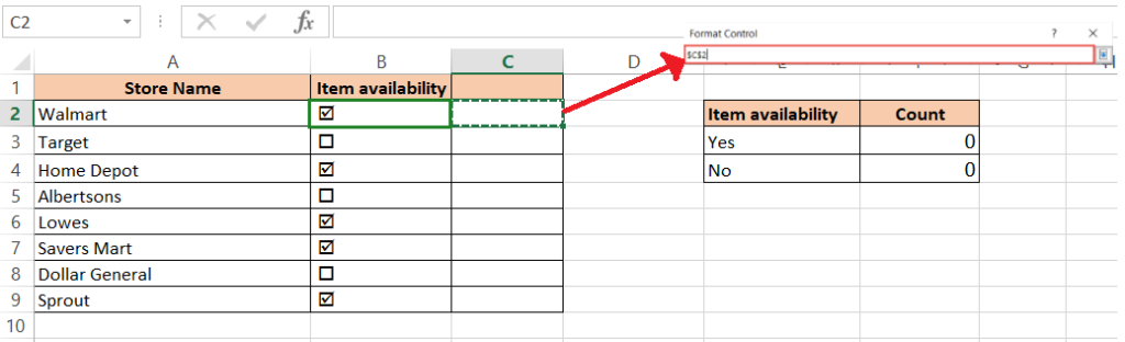
- Click ok to close the dialog box. Now, we can see a TRUE value in the cell C2. We repeat the steps to get a full set of TRUE and FALSE values in the linked cells.
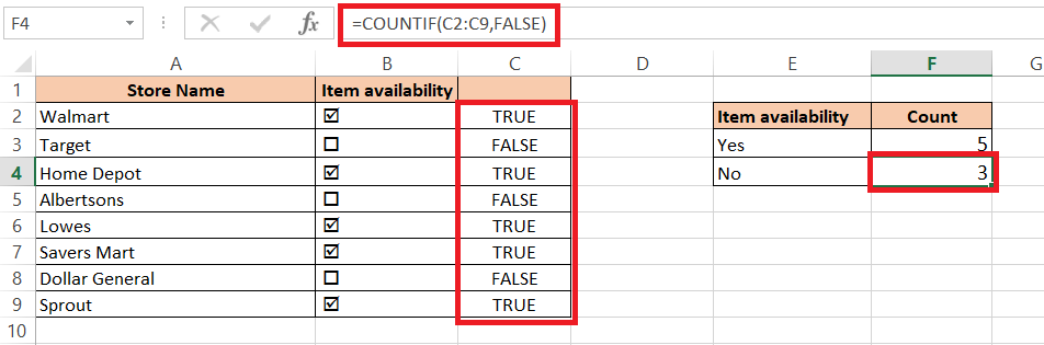
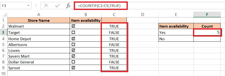
- After all these steps, we will do the main job, which is to count the number of cells that has “TRUE” in it. Let’s insert the following formula in cell F3, as shown below:
- We have to repeat the process for getting the number of cells that has “FALSE” in it.

These are the ways to count the number of “Yes” and “No” in a dataset using the COUNTIF formula.
Hope this tutorial will help you solve your problems in Excel. Stay with us. Thank you!