
Making name lists is a very common task done using Excel. It can be the list of employees, customers, friends, or family members. Sometimes, we may need to extract the last names only to include them in a report.
In this section, we will discuss the ways of extracting last names from excel.
There are 4 easy ways to extract names from Excel.
- The Text-to-columns feature.
- The Flash fill feature.
- Formula.
- Power Query.
We are going to discuss them one by one below. Stay with us!
1. The Text-to-columns feature:
We can separate text in a column into different columns by using the Text-to-columns feature.
This feature works based on a delimiter, which is a character or symbol that separates text in a cell. For example, in a full name, the space character between the first and last names is called delimiter.
The Text-to-column tool is used to separate the first and last names in different columns. Once they are separate columns, we can easily select the column containing first names and delete them and then work with the column that contains only last names.
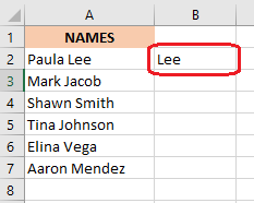
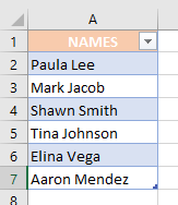
For example, the following table shows some names in the Excel sheet. Let’s see how we separate the last names using the Text-to-columns tool.
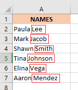
In this picture, the last names are put inside the Red Box so that you can easily identify which part is the last name.
Now, we have to follow the steps below to extract the last names in the picture.
- First, select the list of full names. In the picture, select from cell A2 to A7.
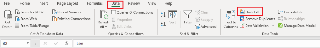
- Then, click “Data” and click “Text to Columns” in the Data Tool box.

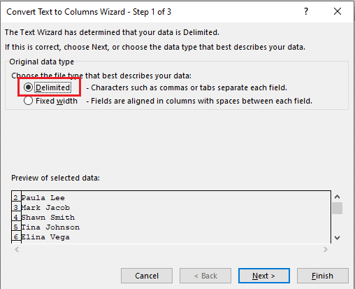
The “Convert text to Columns Wizard” will open. You have to follow 3 steps:
Step-1: check the button “Delimited” as shown in the picture below. Then click the “Next”.
Step- 2: uncheck the box of “Tab” and check the box of “Space”, because we want to separate the first and last names based on the space character.
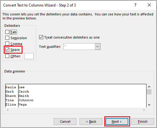
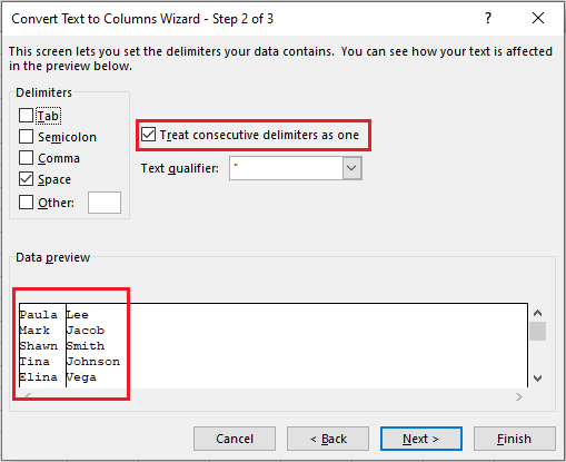
Then, check the box “Treat consecutive delimiter as one” so that excel trims all the extra space characters. (Some names in the list may have more than one consecutive space character, so keep that box checked.)
At the bottom of the Preview box, you will see an example of separating columns of the names. Finally, click “Next”.
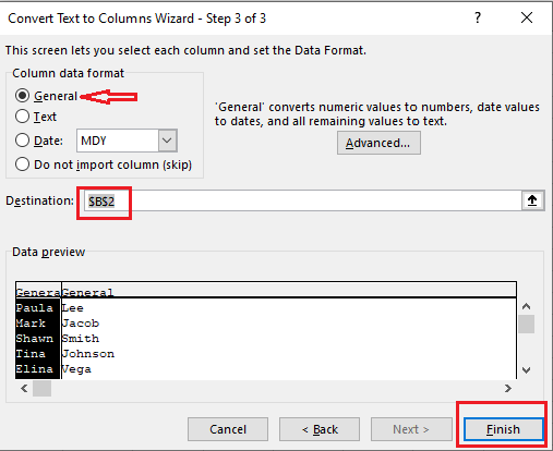
Step- 3: you need to specify the format you want the extracted column to have. To do that check the button “General”.
Write down $B$2 in the input box of the “Destination” so that the separated columns start from Cell B2 (according to the example).
Then, click “Finish”.
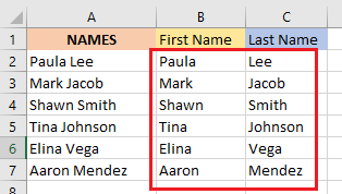
Finally, you will see the names are separated into two separate columns. In the example, first names are in column B and last names are in column C. (write down “First Name” in cell B1 and “Last Name” in cell C1).
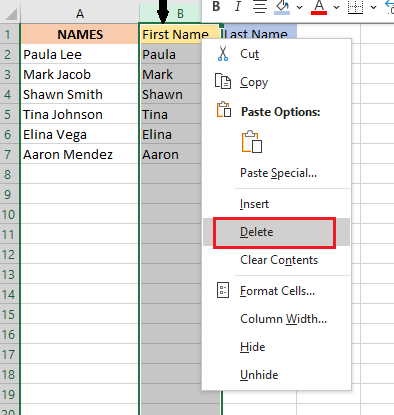
Now select the full column B, press right-click, and select the “delete” option. It will delete the whole column of the first names and transfer the last names in column B.
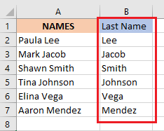
Now you have last names in column B.
Note: If any of the names in the list contains the middle name, the Text-to-column feature will not work. This is because the method only works when all the names have the same segments of names (such as first and last names). If all the names have 3 parts (First, middle, and last names), this method will work. In that case, you have to separate the names into 3 cells.
2. The Flash Fill feature:
The Flash Fill feature is an intelligent feature we find in Excel 2013 or in later versions. It is called intelligent because it recognizes the patterns of the data and automatically fills in the columns based on that pattern.
Unlike the Text-to-columns feature, if some names have middle names, this method recognizes the pattern and easily extracts the last names.
It also copies patterns including capitalizations and punctuations. If the first and last names are separated by commas, this method will recognize that and extract the last names easily.
Following are the steps we can follow to extract the last names from a list of names.
First, write down the last name of the first cell manually in the next cell. For example, we wrote “Lee” in cell B2 manually.
Second, go to “Data” and click on the “Flash Fill” in the Data Tools bar. Alternatively, press the shortcut CTRL+E on the keyboard or Cmd+E for Mac.
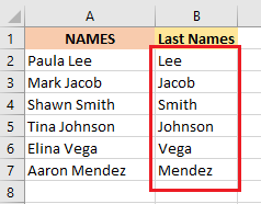
Finally, the list of last names column is filled automatically as shown below.
3. Formulas:
Excel is a great platform to use formulas to solve your problems. To extract last names from a list of names, we can use different formulas. Based on the type of data, we will discuss the formulas.
- When the list has only First and Last names:
The Formula is given below:
=RIGHT(A2,LEN(A2)-SEARCH(” “,A2))
The above formula includes three Functions: RIGHT Function, LEN Function, and SEARCH Function.
(1) The RIGHT Function:
The syntax is:
=RIGHT(text, num_of_characters)
Here,
- “text” means the input string that we want to work on.
- “num_of_character” means number of characters we want to extract from the right side of the text.
Basically, it returns a given number of characters from the right side of a given string.
(2) The LEN Function:
The syntax is:
=LEN(text)
It simply returns the number of characters in a given string.
(3) The SEARCH Function:
The syntax is:
=SEARCH (find_text, within_text, [start_num])
Here,
- “find_text” means the search string, which we want to find.
- “within_text” means the text, which we want search in.
- “start_num” is position in the text where we want to start searching from. Since this parameter ids optional, we can ignore it. Then the search will start from the first position of the text.
This function finds the location of a given string inside another, such as getting the location of a Space character in a given string.
Let’s put the RIGHT, LEN, and SEARCH functions together in the Excel sheet and see how it extracts the last name:
The Formula is:
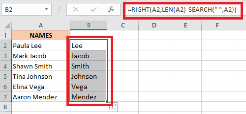
=RIGHT(A2,LEN(A2)-SEARCH(” “,A2))
If we enter the above formula in cell B2 and copy it down to the rest of the cells, we get the following result:
Now we will break down the formula so that you can understand it better.
- SEARCH(” “,A2) returns the position of a space character in the string “Paula Lee” that is in the 6th position in the string.
- LEN(A2)-SEARCH(” “,A2) subtracts the position returned by the SEARCH function from the length of the whole string. “Paula Lee” has 9 strings and the space character is the 6th string, so it returns the value 9 – 6 = 3.
- RIGHT(A2,LEN(A2)-SEARCH(” “,A2)) returns LEN(A2)-SEARCH(” “,A2) character from the right side of the string. In our case, the last 3 character from the string “Paula Lee” is “Lee”.
Note: we can use the FIND function instead of the SEARCH function to get the same result. Moreover, the Trim function can be used to trim out the extra space characters in the names, such as, =TRIM(RIGHT(A2, LEN(A2)-SEARCH(“ “,A2)))
When the list has First, Middle, and Last names:
The formula is different:
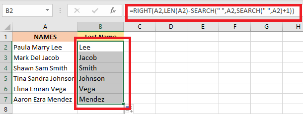
=RIGHT(A2,LEN(A2)-SEARCH(” “,A2,SEARCH(” “,A2)+1))
If we put the above formula in cell B2 and copy it down the cells, we get the following result:
Let’s break down the formula to better understand the function below:
- SEARCH(” “,A2)+1) returns 6, the position of the first space.
- SEARCH(” “,A2,SEARCH(” “,A2)+1) starts searching from the 7th position (6 + 1 = 7), and returns the position of the next space, which is 12th position.
- LEN(A2)-SEARCH(” “,A2,SEARCH(” “,A2)+1) calculates the number of characters in the last name, such as 15 – 12 = 3.
- RIGHT(A2,LEN(A2)-SEARCH(” “,A2,SEARCH(” “,A2)+1)) returns the last 3 characters, which is “Lee”.
When the first and last names are separated by Commas:
In some cases, names are written as Last name, First name. Since the Last name in on the left side, we have to use the Left function.
The LEFT function returns a given number of characters from the left side of the string. The syntax is:
LEFT(text, num_of_characters)
Here, “text” is the input string that we want to work on, and “num_of_characters” is the number of characters that we want to extract from the left side of the text.
Let’s see the formula for the last names separated by commas:
=LEFT(A2,SEARCH(“, “,A2)-1)
Now, if we apply the formula in cell B2 and copy it down to the other cells, we get following result:
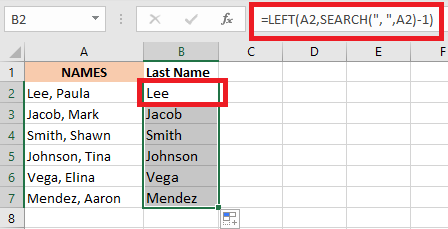
We can see that the formula extracted names from the left side before the comma that are basically the last names.
Let’s break down the above formula to better understand how it works.
- SEARCH(“, “,A2) returns the position of comma character in the string “Lee, Paula”. Since the comma is in the 4th position in the string, it returns number 4.
- LEFT(A2,SEARCH(“, “,A2)-1) returns 4 – 1 = 3 character from the left side of the string. In the example, the 3 characters from the left side is “Lee”.
4. Power Query:
In the newer version of Excel, the power query can be found in Data tool section. But in an older version of Excel, we have to install it as an add-in. It is a great tool, which also includes functions like splitting and merging columns.
Let’s discuss the steps of the power query below:
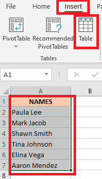
(a) The first step is to convert the list of names into an Excel table. To do that, we will select the data, then go to Insert and click Table (Alternatively, press the shortcut CTRL+T).
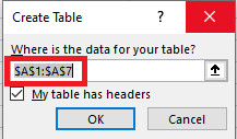
(b) Then the Create Table dialog box will appear where we have to make sure that the data range is correct. For example, A1:A7.
(c) Now we can see our data in a table.
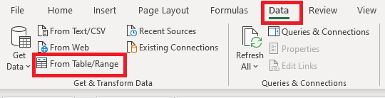
(d) To use a power query in the data, select any cell in the table. Then select “From Table/Range” in the Data section (in the Get & Transform section).
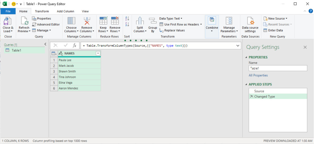
(e) Following power query editor box will appear.
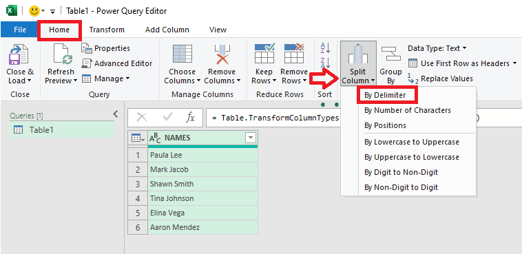
(f) In the editor box, got o Home, Click “Split Column” and click “ By Delimiter”.
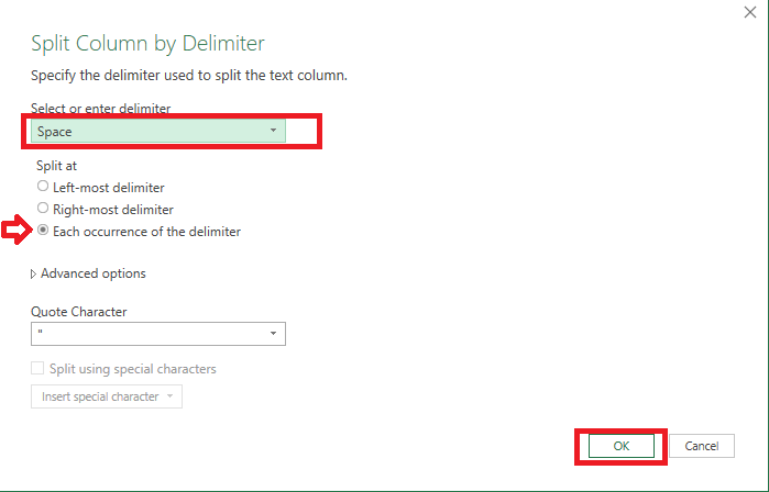
(g) “Split Column by Delimiter” dialog box will open.
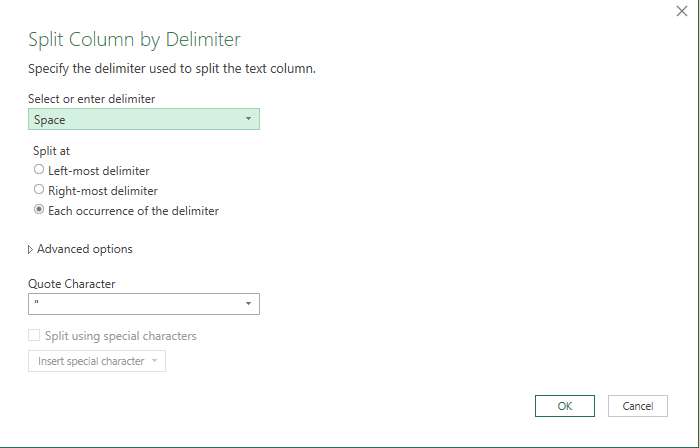
(h) We need to make sure that the space option is selected and the “Each Occurrence of the Delimiter” is selected too. Then click “OK” button.
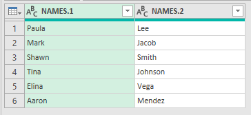
(i) Now we can see two splitting tables, one includes first names and the other includes last names.
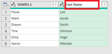
(j) To change the column header, we have to double click the column header and change it to “Last Name”, as shown below.
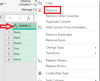
(k) Alternatively, we can right-click on the first name column header and select “Remove” in order to delete the first name table altogether.
(l) Now, from the File tab click “Close & Load”.
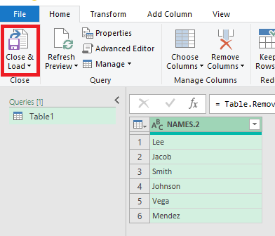
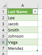
(m) Finally we will get a new sheet in our workbook that contains a table of last names.
Note: we can retain the original name table by creating a duplicate table for this function. To do that, select “Add Column” tab in the Power Query Editor and select “Duplicate Column”.
Although the Power Query involves too many steps and seems complicated, it is the best way to extract last names in the long run. You can avoid repeating all these steps for a new worksheet simply by adding it to the power query data cleaning process.
Hope this article will help solve your problem. Thank you!