Currency vs Accounting Format in Excel
Both Currency and Accounting styles are formatting styles that Excel uses to display numbers in cells. To understand the difference between currency vs accounting format in Excel, let’s take a look at the examples below.
Currency vs Accounting Format
1. Select the range of cells C3:C8.
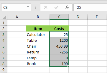
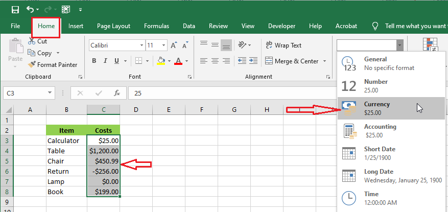
2. Apply “Currency format” from the Home tab.
3. Now, apply “Currency format” from the Home tab.
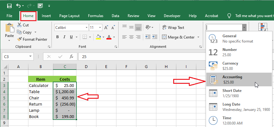
Note: The difference between them is that (1) Currency style puts a dollar sign at the front of each number without alignment, (2) Accounting style puts a dollar sign at the front of each number and aligns them. Additionally, negative numbers are in parathesis, and zero values or displayed as hyphens.
Displaying negative numbers
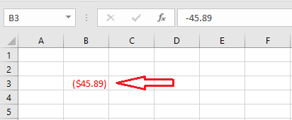
To display a negative number using currency style (e.g., display in red and negative sign in front).
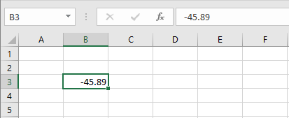
1. Enter -45.89 in cell B3.
2. Select cell B3.
3. Right-click and select “Format Cell.”
4. From the category, select “Currency” and highlight the last options from the “Negative numbers:”.
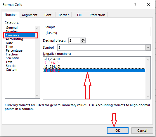
5. Click OK.
Displaying Finacial Statement Style
In a financial statement, you often see numbers displayed with a single or double underline. Here is how to apply this style.
1. Select cell B3 as in the previous picture.
2. Right-click and select “Format Cell.”
3. From the Font tab, select “Single Accounting” style from the drop-down list.

4. Click OK.
Result:
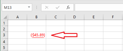
Note: Now, try out the “Double Accounting” style and see what this number looks like.
| 4 of 14 finished! Recommending more on Format Cells: Next Example >> |
| << Previous Example | Skip to Next Chapter 05: Formulas and Functions Basics |