Display Numbers as Fractions in Excel

To learn how to display numbers as fractions in an Excel cell and how to change the format of a fraction, follow the steps below.

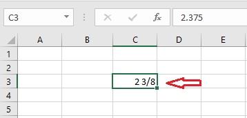
1. Select cell C3 and type either 2 3/8 or 0 3/8 as a mixed fraction.

Note that excel changed the cell’s format in the background. The formula bar shows the fraction, but the cell shows exactly what you have typed in.

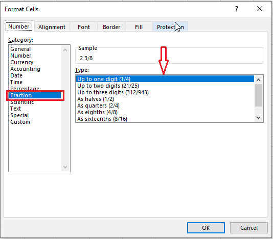
2. To check what format style cell C3 has, select cell C3, right-click, and select “Format Cells.”

Note: excel shows “Up to one digit” style.

3. Now, type in 2 4/111 in cell C3.

Note: Excel shows the denominator rounded two. In other words, Excel reduces the fraction to its smallest denominator. Excel automatically sets the type as “Up to two digits (21/25).”

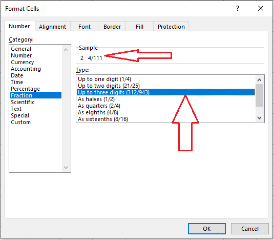
4. To change to “Up to three digits..”, select cell C3, right-click, and select “Format Cells.”

5. Select “Up to three digits ….”

6. Click OK.

Now you get to see the number that you typed in the first place.

Note: We recommend you play around with different combinations of these styles in Excel. You will definitely understand better how these styles work.

3 of 14 finished! Recommending more on Format Cells: Next Example >>

<< Previous Example | Skip to Next Chapter 05: Formulas and Functions Basics