Excel Freeze Panes
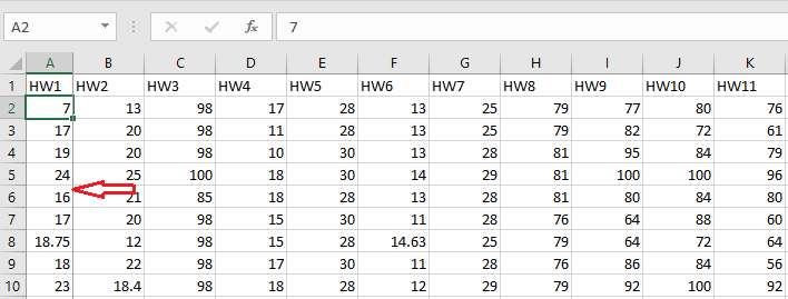
When you work with a large table of data in Excel, the freeze panes allows you to freeze rows or columns for better visibility. In other words, you can keep one part of the table visible while scrolling up or down the other part.
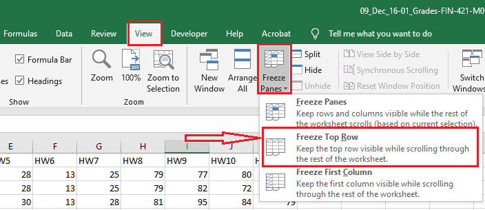
Freeze Top Row
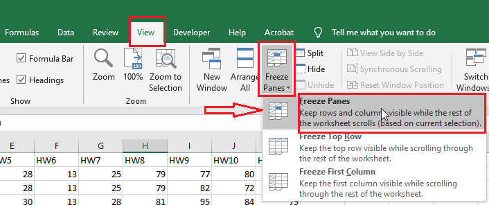
1. Click “Freeze Panes” on the View tab. Select Freeze Top Row.
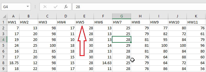
2. Now, if you scroll down the worksheet, you notice that Excel adds a horizontal line right below the top row, which is frozen.
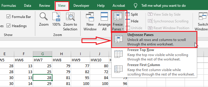
Unfreeze Panes
1. To unfreeze, click “Freeze Panes” on the View tab.
2. Click “Unfreeze Panes.”
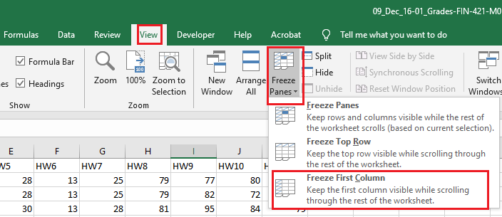
Freeze First Column
1. Click “Freeze Panes” on the View tab.
2. Click “Freeze First Column.”
3. Now, if you scroll to the right, you notice that Excel adds a vertical line right after the first column, which is frozen.
Freeze Rows
1. Select Row 5.
2. Click “Freeze Panes” on the View tab.
3. Click “Freeze Panes.”
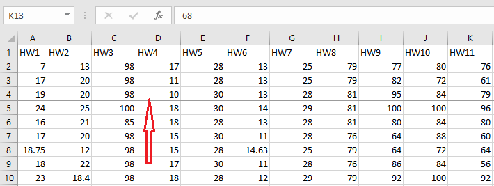
4. Now, you notice that Excel adds a horizontal line right above row 5. All rows above row 5 are frozen.
Freeze Columns
1. Select column C.
2. Click “Freeze Panes” on the View tab.
3. Click “Freeze Panes.”
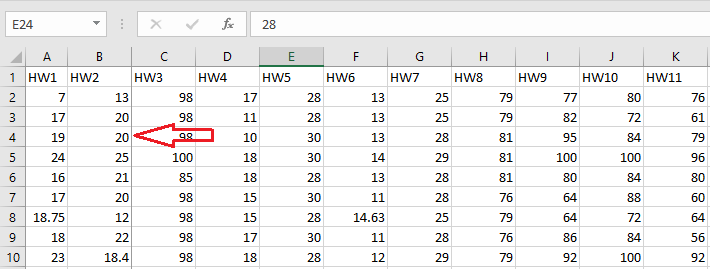
4. Now, you notice that Excel adds a vertical line right before column C. All columns before column C are frozen.
Freeze Cells
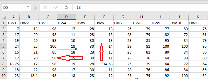
1. Select cell D5.
2. Click “Freeze Panes” on the View tab.
3. Click “Freeze Panes.”
4. Now, you notice that Excel adds a vertical line and a horizontal line to the top and left of cell D5. Areas above row 5 and left of column D are frozen.
Add Freeze Button
If you frequently need to freeze rows, columns, or cells, it is useful to add the Freeze button to the Quick Access Tool Bar. In this way, you can just open the Freeze Pane with a single mouse click.
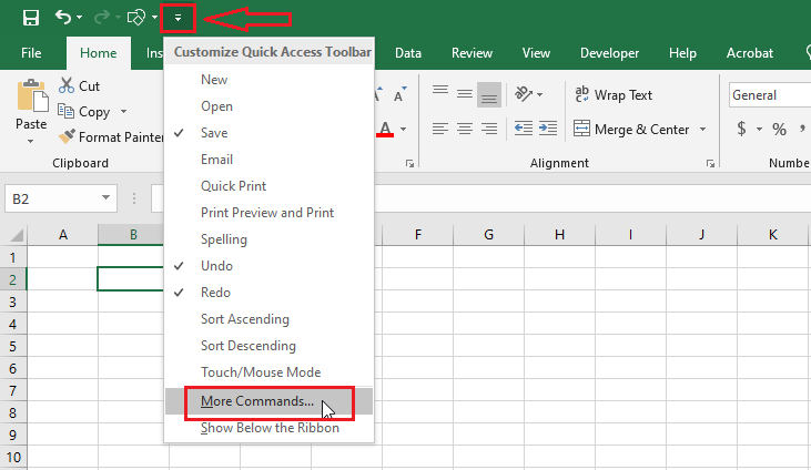
1. Click on the little down arrow.
2. Click “More Commands.”
3. Select “Commands Not in the Ribbon” under the “Choose commands from.”
4. Now, scroll down and select the “Freeze Panes” command and click Add.
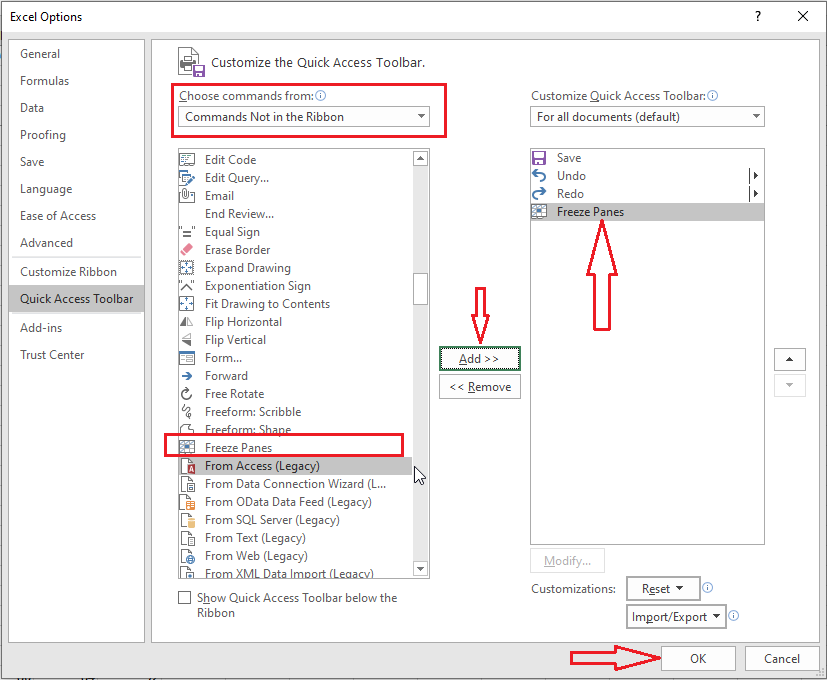
5. Click OK.
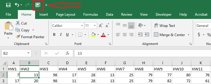
Note: If you like to use this Quick Access Tool Bar icon, just click on the icon and Excel will automatically freeze the areas depending on the cell you selected.
| 4 of 9 finished! Recommending more on Worksheet: Next Example >> |
| << Previous Example | Skip to Next Chapter 05: Formatting Cells |