Create a Meal Chart in Excel
In this lesson, we will create a weekly meal chart or planner in Excel from the scratch. To accomplish this goal, follow the steps below.
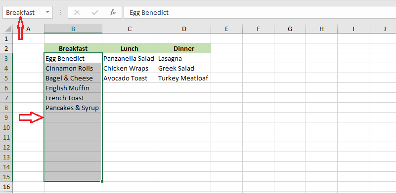
1. In Sheet2, we Named Range B3:B15 as Breakfast, C3:C15 as Lunch, and D3:D15 as Dinner.
2. In Sheet1, select cell C5.
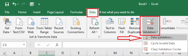
3. From the Data tab, click “Data Validation”.
4. In Allow box, select List from the drop-down list.
5. In the Source box, type in =Breakfast.
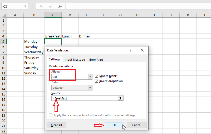
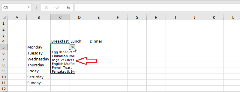
6. Click OK and get the following result.
7. Repeat steps 2 to 6 for cells D5 (Lunch) and E5 (Dinner).
8. Select the range C5:E5. Using the fill handle, drag it down to cell E11.
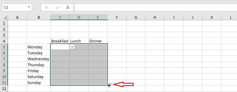
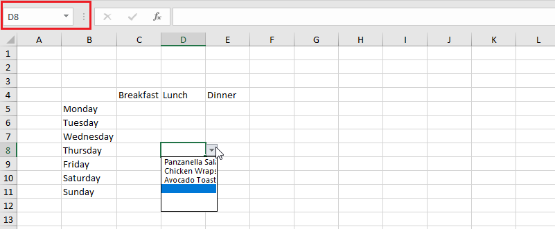
9. Now, click anywhere within the range C5:E11. You should see the drop-down list with your respective food items.
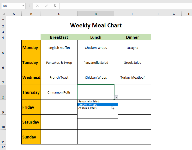
10. Now, you can uncheck the grid line on the View tab and other formatting styles as you like. For instance, we have applied different font sizes, highlights, and cell border styles as given below.
Note: To download our version of the weekly meal planner and compare it with yours, click HERE.
| 3 of 5 finished! Recommending more on Find and Select: Next Example >> |
| << Previous Example | Skip to Next Chapter 10: Keyboard Shortcuts |