Transpose Data in Excel
We can transpose data in Excel using the “Paste Special” option or the TRANSPOSE function to switch rows to columns or vice-versa.
Using Paste Special
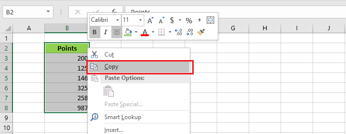
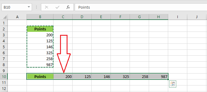
1. To switch the column to a row, select the range B2:B8.
2. Right-click and click copy.
3. Select cell B10. Right-click and then click Paste Special.
4. From the Paste Special dialog box, check Transpose.
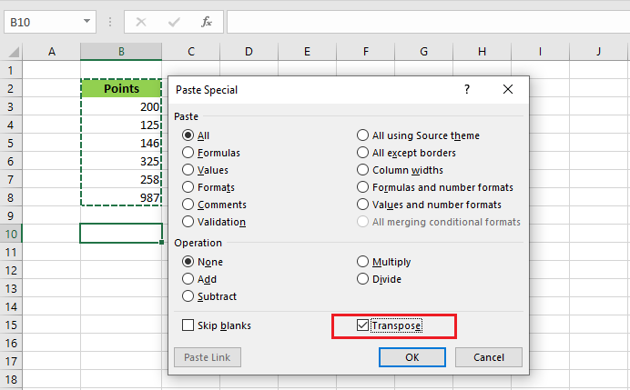
5. Click OK.
Using Transpose Function
While using the “Paste Special” option in transposing Excel data serves your purpose, the transposed data does not update automatically when changing the source data. The TRANSPOSE function overcomes this issue. Let’s take a look at the examples below.
1. To switch the row to a column, select the new range of cells (B3:B8).
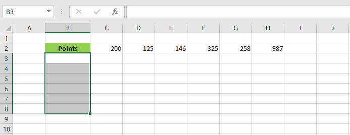
2. Now, type in =TRANSPOSE(
3. Select the range C2:H2 and close the parenthesis.
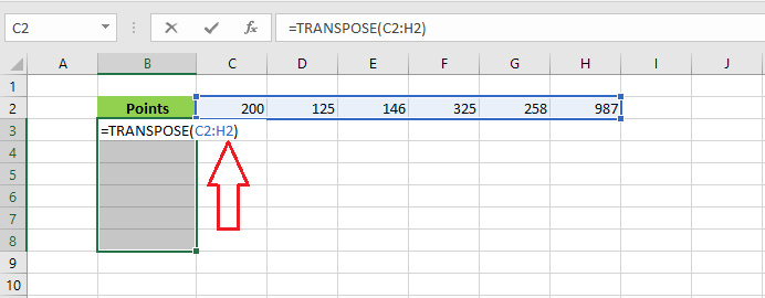
4. Finally, press CTRL+SHFT+ENTER.
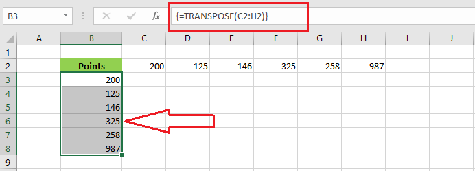
Note: the formula in the formula bar is enclosed with curly braces, { }, indicating that it is an array formula.
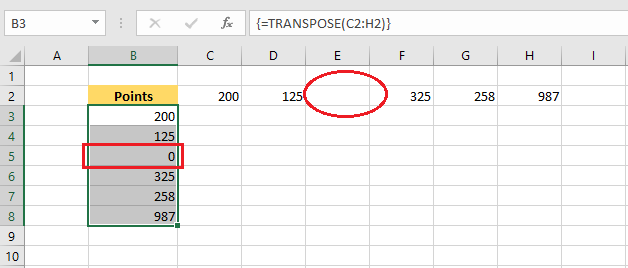
Transpose Data with Blank Cell
1. Cell E2 below is blank. The TRANSPOSE function converts this missing information into a zero.
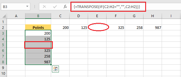
2. If you like the TRANSPOSE function returns a blank instead of zero, write an IF function inside the transpose function. The resulting output is given below.
| 5 of 12 finished! Recommending more on the Range: Next Example >> |
| << Previous Example | Skip to Next Chapter 03: Understanding Workbook |