Hide Columns and Rows in Excel
You can right-click and select the “hide” option to hide columns and rows in Excel. Follow the steps below.
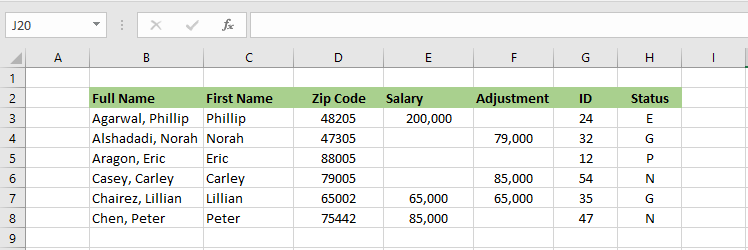
Hide
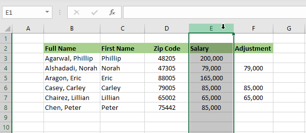
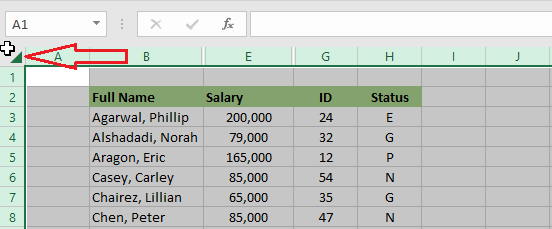
1. Select a column as in the picture.
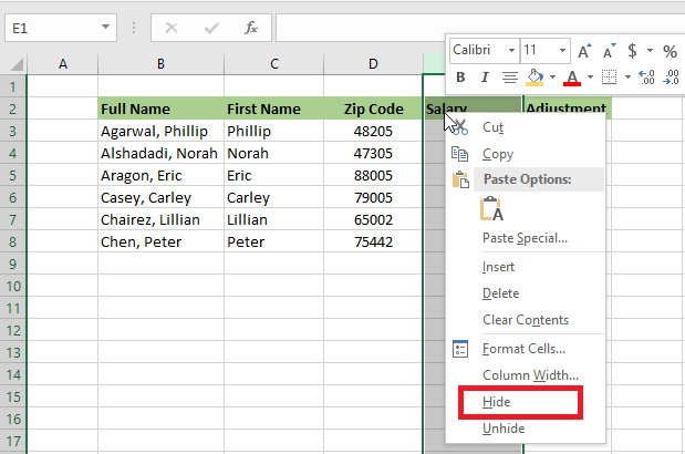
2. Right click and click “Hide.”
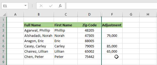
Result:
Let’s unhide what you have just hidden.
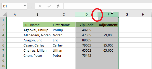
3. Select the columns on both sides of the hidden column.
4. Right click on your mouse and then click “Unhide.”
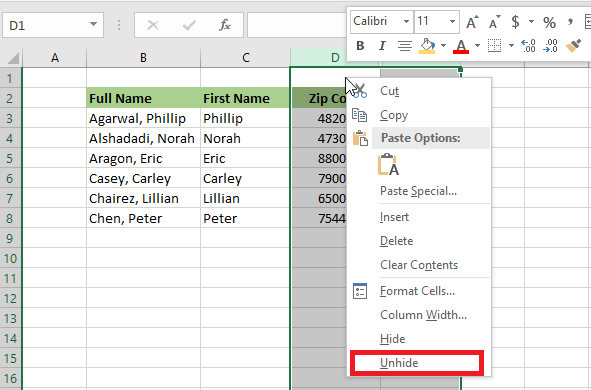
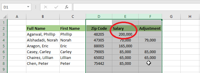
Result:
Note: To hide or unhide a row, follow the same steps as above.
Hide Multiple Columns
1. To hide multiple columns, select the columns by their heads. Please note that you can also select non-adjacent columns by holding down CTRL and clicking the column head of your choice. In the picture below, columns C, D, and F are selected.
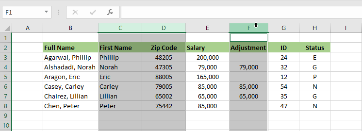
2. As shown ins step 4 above, right click on your mouse and then click “Hide.” You get the following result.
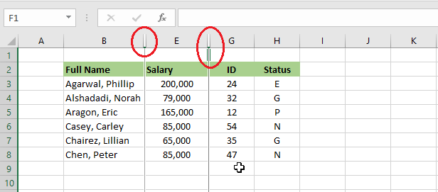
3. To unhide, select all the columns by clicking the triangular button at the corner of the sheet.
4. Right click and then click “Unhide.” The result is given below.
Note: To hide or unhide multiple rows, you follow the same steps as above.
Hide Columns using Group option
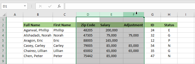
1. Select columns that you want to hide.
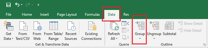
2. Go to Data tab and click “Group.”
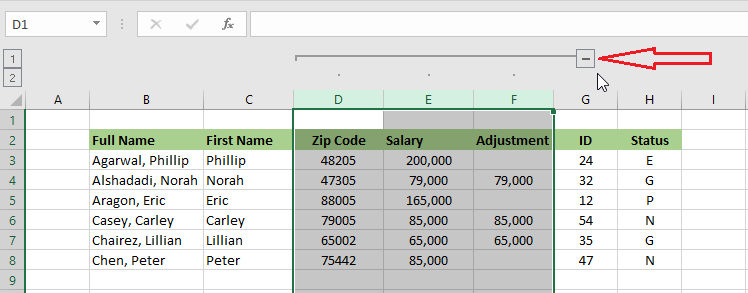
3. Click the minus button to hide columns.
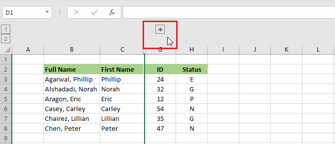
4. Click the plus button to unhide columns.
Note: To ungroup the columns, select the columns that were grouped and then select “Ungroup” in the Data tab.
Hide Data in Cells
To hide data in cells, follow these steps.
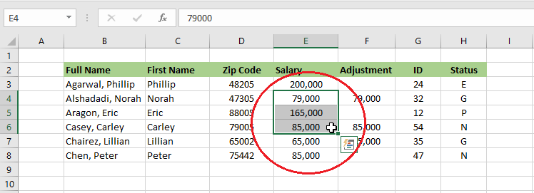
1. Select the cells that you want to hide the data of.
2. Right click and then click “Format Cells.”
3. In the dialog box, click “Custom.”
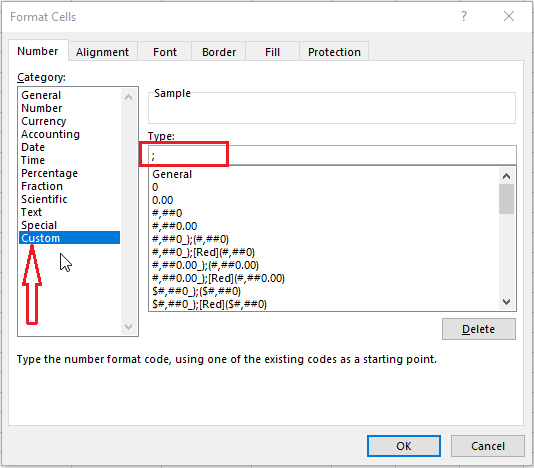
4. Now, type a semicolon (;) and then click OK.
Result:
Note: the data in the cells (E4:E6) is just invisible. If you select any of these hidden cells and look at the formula bar, you are going to see the data. To unhide the information, just reverse the process.
| 9 of 12 finished! Recommending more on the Range: Next Example >> |
| << Previous Example | Skip to Next Chapter 03: Understanding Workbook |